Probabilities & Bayes rule (in memo)

Author: Michael Franke, adapted to memo by Robert D. Hawkins

In this appendix, we’ll introduce the basic tools of probability and Bayesian reasoning using memo, a probabilistic programming language designed for modeling how people reason about other agents.

Getting started with memo

Programming languages are formal systems for describing computations. Traditional (imperative) programming languages are designed for deterministic computations. You can always implement probabilistic models in a traditional programming language. But this gets quite cumbersome for more complex models. It’s much better to work in a probabilistic programming language (PPL) like memo that provides elegant abstractions for building and manipulating probability distributions, allowing us to write generative models with built-in uncertainty.

memo is a domain-specific probabilistic programming language designed specifically for modeling reasoning about reasoning (Chandra et al., 2025). It has some features that make it particularly well-suited for modeling the kinds of sophisticated reasoning processes involved in computational pragmatics and language understanding.

Agents and observers: memo makes explicit the distinction between different reasoning agents. You can model an observer who has certain beliefs about how a friend or agent makes decisions. This is crucial for keeping track of who knows what.

Recursive reasoning: The language naturally expresses hierarchical reasoning structures where agents reason about other agents’ reasoning. For example, an observer can model what a friend thinks about a third party’s beliefs.

Declarative syntax: memo uses a declarative syntax that closely mirrors how cognitive scientists think about mental models. Rather than writing code manually implementing inference, you simply declare the structure of agents’ beliefs and reasoning processes.

Integration with JAX: memo is built on top of JAX, providing automatic differentiation and GPU acceleration for scalable probabilistic computation.

In this section, we’ll work through several examples that demonstrate key concepts in probability and Bayesian reasoning. These examples are drawn from the course notes for “Computational Models of Social Cognition” by Dae Houlihan.

Example 1: Enumerating over outcomes

Before diving into complex probabilistic reasoning, let’s understand how memo works at the most basic level. Here’s the simplest possible memo program:

import jax
import jax.numpy as jnp
from enum import IntEnum
from memo import memo

class Coin(IntEnum):
    TAILS = 0
    HEADS = 1

@memo
def coin_outcomes[_c: Coin]():
    return _c

res = coin_outcomes(print_table=True)

What’s happening here?

• The @memo decorator tells Python this is a probabilistic program written in memo
• [_c: Coin] means this model will enumerate over the Coin values and call them _c
• The function returns a table with all possible outcomes of the coin flip.

this demonstrates memo’s basic enumeration mechanism - rather than calling the function with specific arguments, memo considers all possible arguments and their outcomes.

Example 2: Computing a distribution

What makes memo a probabilistic programming language is that it natively builds probability distributions. To take this it for a spin, we’ll model an agent (called observer) who makes random choices and compute probabilities over those choices.

@memo
def coin_flip_prior[_c: Coin]():
    observer: given(c in Coin, wpp=1)
    return Pr[observer.c == _c]

res = coin_flip_prior(print_table=True)

This function computes the probability of each coin outcome. Since we have a uniform distribution over two outcomes, each should have probability 0.5. The syntax observer: given(c in Coin, wpp=1) creates an observer agent who samples a value c from the Coin domain. The wpp=1 means “with probability proportional to 1” - since both coin values get the same weight, this creates a uniform distribution. The Pr[observer.c == _c] syntax asks: “What’s the probability that the observer’s coin choice equals the value _c?” By convention, we will write variables with underscores like _c to indicate that these are the values we’re building the distribution over.

Example 3: Events

Now let’s consider flipping two coins and computing the probability that at least one comes up heads.

from memo import domain as product

SampleSpaceTwoFlips = product(
    f1=len(Coin),
    f2=len(Coin),
)

@jax.jit
def sumflips(s):
    return SampleSpaceTwoFlips.f1(s) + SampleSpaceTwoFlips.f2(s)

@memo
def flip_twice():
    observer: given(s in SampleSpaceTwoFlips, wpp=1)
    return Pr[sumflips(observer.s) >= 1]

flip_twice(print_table=True)

Example 4: More complex events

For a more complex example, let’s flip 10 coins and compute the probability of getting between 4 and 6 heads (inclusive):

nflips = 10
SampleSpace = product(**{f"f{i}": len(Coin) for i in range(1, nflips + 1)})

@jax.jit
def sumseq(s):
    return jnp.sum(jnp.array([SampleSpace._tuple(s)]))

@memo
def flip_n():
    student: given(s in SampleSpace, wpp=1)
    return Pr[sumseq(student.s) >= 4, sumseq(student.s) <= 6]

flip_n(print_table=True)

The 3-card problem: motivating Bayesian reasoning

Jones is not a magician or a trickster, so you do not have to fear. He just likes probability puzzles. He shows you his deck of three cards. One is blue on both sides. A second is blue on one side and red on the other. A third is red on both sides. Jones shuffles his deck, draws a random card (without looking), selects a random side of it (without looking) and shows it to you. What you see is a blue side. What do you think the probability is that the other side, which you presently do not see, is blue as well?

Many people believe that the chance that the other side of the card is blue is .5; that there is a 50/50 chance of either color on the back. After all, there are six sides in total, half of which are blue, and since you do not know which side is on the back, the odds are equal for blue and red.

This is faulty reasoning. It looks only at the base rate of sides. It fails to take into account the observation-generating process, i.e., the way in which Jones manipulates his cards and “generates an observation” for you. For the 3-cards problem, the observation-generating process can be visualized as in Fig. 1.

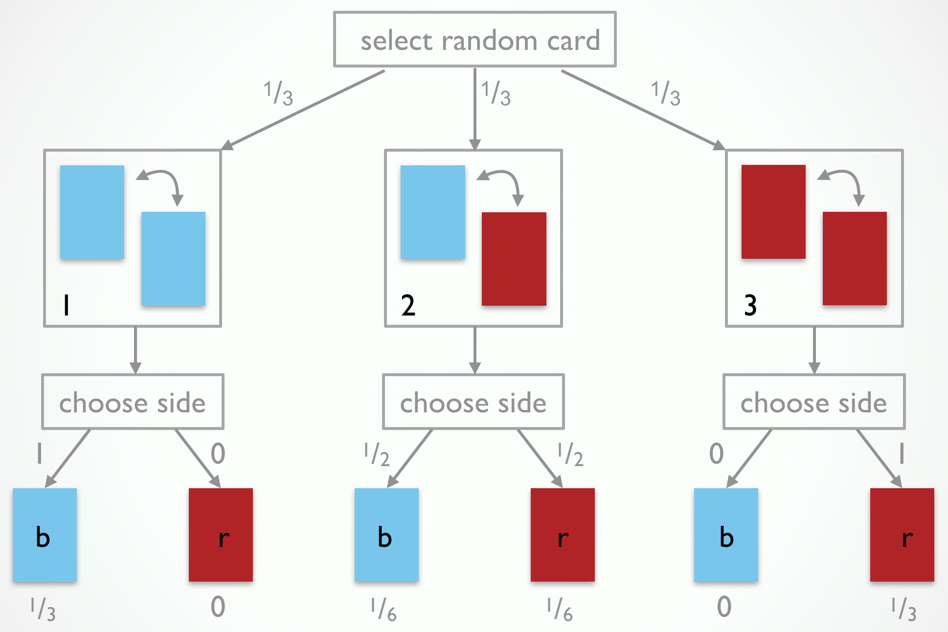
The process tree in Fig. 1 also shows the probabilities with which events happen at each choice point during the observation-generating process. Each card is selected with equal probability \(\frac{1}{3}\). The probability of showing a blue side is 1 for the blue-blue card, .5 for the blue-red card, and 0 for the red-red card. The leaves of the tree show the probabilities, obtained by multiplying all probabilities along the branches, of all 6 traversal of the tree (including the logically impossible ones, which naturally receive a probability of 0).

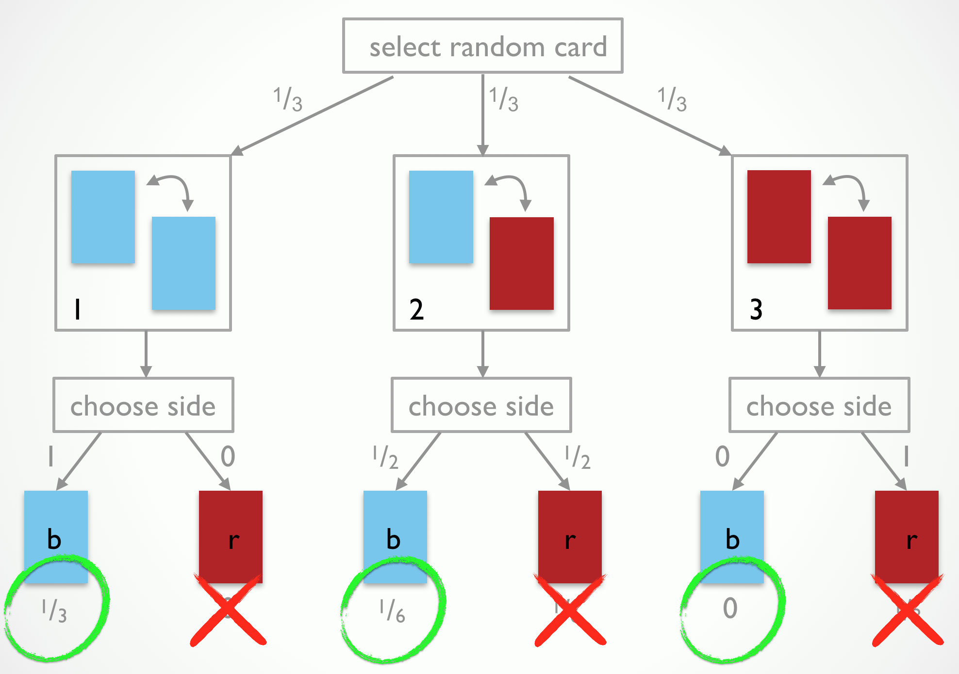
If we combine our knowledge of the observation-generating process in Fig. 1 with the observation that the side shown was blue, we should eliminate the outcomes that are incompatible with it, as shown in Fig. 2. What remains are the probabilities assigned to branches that are compatible with our observation. But they do not sum to 1. If we therefore renormalize (here: division by .5), we end up believing that it is twice as likely for the side which we have not observed to be blue as well. The reason is because the blue-blue card is twice as likely to have generated what we observed than the blue-red card is.

The latter reasoning is actually an instance of Bayes rule. For our purposes, we can think of Bayes rule as a normatively correct way of forming (subjective) beliefs about which causes have likely generated an observed effect, i.e., a way of reasoning probabilistically and defeasibly about likely explanations for what has happened. In probabilistic pragmatics we will use Bayes rule to capture the listener’s attempt of recovering what a speaker may have had in mind when she made a particular utterance. In other words, probabilistic pragmatics treats pragmatic interpretation as probabilistic inference to the best explanation of what worldly states of affairs, mental states and contextual factors would have caused the speaker to act in the manner observed.

You should now feel very uncomfortable. Did we not just say that most people fail at probabilistic reasoning tasks like the 3-card problem? (Other prominent examples would be the two-box problem or the Monty Hall problem.) Yes, we did. But there is also a marked contrast between probability puzzles and natural language understanding. One reason for why many people fail to show the correct probabilistic reasoning in the 3-card problem is because they neglect the precise nature of the observation-generating process. The process by which Jones selects his cards is not particularly familiar to us. (When is the last time you performed this card selection procedure.) In contrast, every speaker is intimately familiar with the production of utterances to express ideas. It is arguably a hallmark of human language that we experience ourselves in the role of the producer (compare Hockett’s design features of language, in particular total feedback). On this construal, pragmatic interpretation is (in part) a simulation process of what we might have said to express such-and-such in such-and-such contextual conditions.

Probability distributions & Bayes rule

If \(X\) is a (finite) set of mutually discrete outcomes (results of an experiment, utterances, or interpretations), a (discrete) probability distribution over \(X\) is a function \(P \colon X \rightarrow [0;1]\) such that \(\sum_{x \in X} P(x) = 1\). For any subset \(Y \subseteq X\) we further define \(P(Y) = \sum_{x \in Y} P(x)\).

Consider the example of a 2-dimensional probability table. It gives probabilities for meeting a person with a particular hair and eye color.

Formally, we have \(X = H \times E\) with \(H = \{ \text{black}, \text{blond}, \text{red} \}\) and \(E = \{ \text{brown}, \text{blue}, \text{green} \}\). The probability of meeting a person with black hair and green eyes would accordingly be \(P(\langle \text{black}, \text{green} \rangle) = .01\).

Denote with \(\text{"black"}\) the proposition of meeting a person with black hair. This is a subset of the outcome space: \(\text{"black"} = \{ \langle h , e \rangle \in X \mid h = \text{black} \}\). Similarly, for other hair and eye colors. The probability of meeting a person with black hair is obtained by marginalization: \(P(\text{"black"}) = .4 + .02 + .01 = .43\).

If \(A, B \subseteq X\) with \(B \neq \emptyset\), the conditional probability of \(A\) given \(B\) is

For example, the conditional probability of a person to have black hair given that she has green eyes is:

A direct consequence of this definition is Bayes rule which relates the conditional probability of \(A\) given \(B\) to the conditional probability of \(B\) given \(A\):

Bayes rule is most useful for abductive reasoning to the best explanation of an observation (effect) based on some unobservable cause. Consider the 3-card problem again. We would like to infer which card Jones selected based on what we saw (i.e., only one side of it). In other words, we would like to know the conditional probability of, say the blue-blue card, given that we have observed one blue side: \(P(\text{blue-blue} \mid \text{obs. blue})\). What we have is an observation-generating process that specifies the reverse, namely the conditional probability of observing blue or red, given a card. Formally, we would get:

Let’s write out this computation in “base” Python and check the results:

import jax
import jax.numpy as jnp
import xarray as xr

from enum import IntEnum

class Color(IntEnum):
    RED = 0
    BLUE = 1

class Card(IntEnum):
    RED_RED = 0
    RED_BLUE = 1
    BLUE_BLUE = 2

class Side(IntEnum):
    FIRST = 0
    SECOND = 1

# Define the card-side color matrix upfront
card_colors = jnp.array([
        [Color.RED, Color.RED],      # RED_RED card
        [Color.RED, Color.BLUE],     # RED_BLUE card  
        [Color.BLUE, Color.BLUE]     # BLUE_BLUE card
    ])

@jax.jit
def check_color(card, side):
    return card_colors[card][side]

def color_prior(color):
    # Count how many of the total sides have this color 
    return jnp.sum(card_colors == color) / card_colors.size

def card_prior(card):
    # Assume a uniform prior over cards
    return 1 / len(Card)

def card_posterior(card, color):
    # P(color | card): proportion of sides on this card that match the color
    likelihood = jnp.mean(card_colors[card] == color)
    
    # P(card): look up prior probability of selecting this card
    prior = card_prior(card)
    
    # P(color): look up marginal probability of the color
    evidence = color_prior(color)
    
    # Bayes' rule: P(card | color) = P(color | card) * P(card) / P(color)
    return (likelihood * prior) / evidence

# Calculate and display prior probabilities
print("Prior probabilities of colors:")
print(f"P(RED) = {color_prior(Color.RED):.4f}")
print(f"P(BLUE) = {color_prior(Color.BLUE):.4f}")

# Display the full probability table
print("\nFull probability table:")
print("Card | Side 1 | Side 2")
print("----------------------")
for card in cards:
    side1 = "RED" if check_color(card, 0) == Color.RED else "BLUE"
    side2 = "RED" if check_color(card, 1) == Color.RED else "BLUE"
    print(f"{card+1:4d} | {side1:6s} | {side2:6s}")

# Calculate and display posterior probabilities
print("\nPosterior probabilities of cards given color:")
print("\nGiven RED:")
for card in cards:
    print(f"P(card {card+1} | RED) = {card_posterior(card, Color.RED):.4f}")
print("\nGiven BLUE:")
for card in cards:
    print(f"P(card {card+1} | BLUE) = {card_posterior(card, Color.BLUE):.4f}")

Example 5: The 3-card problem

Now we’re ready to tackle the 3-card problem using memo. Recall our setup: Jones has three cards (red-red, red-blue, blue-blue), randomly selects one, randomly chooses a side, and shows you a blue side. What’s the probability that the hidden side is also blue? Before seeing any evidence, let’s compute the probability of seeing each color. We model an agent who randomly selects a card and a side:

class Color(IntEnum):
    RED = 0
    BLUE = 1

class Card(IntEnum):
    RED_RED = 0
    RED_BLUE = 1
    BLUE_BLUE = 2

class Side(IntEnum):
    FIRST = 0
    SECOND = 1

# Define the card-side color matrix upfront
card_colors = jnp.array([
        [Color.RED, Color.RED],      # RED_RED card
        [Color.RED, Color.BLUE],     # RED_BLUE card  
        [Color.BLUE, Color.BLUE]     # BLUE_BLUE card
    ])

@jax.jit
def check_color(card, side):
    return card_colors[card][side]

@memo
def color_prior[_c: Color]():
    agent: given(card in Card, wpp=1)
    agent: given(side in Side, wpp=1)
    return Pr[check_color(agent.card, agent.side) == _c]

print("Prior probabilities of colors:")
color_prior(print_table=True)

So far we haven’t inferered anything, we’ve just set up a prior distribution. This is sometimes called the “forward model” or the “generative model”. Now for the key question: given that we observed a blue side, what’s the probability each card was selected? This is where memo’s power really shines. We can model this as an observer reasoning about what a friend (Jones) was thinking when they see the card:

@memo
def card_posterior[_card: Card, _color: Color]():
    observer: knows(_card, _color)
    observer: thinks[
        friend: chooses(card in Card, wpp=1),
        friend: chooses(side in Side, wpp=1),
        friend: given(color in Color, 
                        wpp=color==check_color(card, side))
    ]
    observer: observes [friend.color] is _color
    return observer[Pr[friend.card == _card]]

print("\nPosterior probabilities:")
res = card_posterior(print_table=True, return_aux=True, return_xarray=True)

# Extract and display the results more clearly
xa = res.aux.xarray
pr_red = xa.loc[:, 'RED']
pr_blue = xa.loc[:, 'BLUE']

print(f"\nGiven we observed RED:")
print(f"        P(card 1 | RED) = {pr_red.loc[0].sum():.4f}")
print(f"        P(card 2 | RED) = {pr_red.loc[1].sum():.4f}")
print(f"        P(card 3 | RED) = {pr_red.loc[2].sum():.4f}")

print(f"\nGiven we observed BLUE:")
print(f"        P(card 1 | BLUE) = {pr_blue.loc[0].sum():.4f}")
print(f"        P(card 2 | BLUE) = {pr_blue.loc[1].sum():.4f}")
print(f"        P(card 3 | BLUE) = {pr_blue.loc[2].sum():.4f}")

The observer: thinks[...] block models the observer’s expectations about how Jones (the friend) makes decisions (in this case, drawing cards and sides randomly). The observer: observes [friend.color] is _color line represents conditioning on the observation. Notice how the posterior probabilities match our earlier calculations - the blue-blue card (card 3) is twice as likely as the red-blue card (card 2) when we observe blue!